Multithreading and Map-Reduce in Stan
Stan Map-Reduce
Stan allows you to split your data into shards, calculate the log likelihoods for each of those shards, and then combine the results by summing and incrementing the target log density.
Stan’s map function takes an array of parameters thetas, real data x_rs, and integer data x_is. These arrays must have the same size.
Example
This is a re-implementation of Richard McElreath’s multithreadign and map-reduce with cmdstan using Rstan instead of cmdstan. Additionally, I show how you can have the number of shards as an input instead of hard-codding it.
Makevars
Before you run anything make sure your Makevars has the correct flags. To edit it you can just run usethis::edit_r_makevars()
CXX14FLAGS = -DSTAN_THREADS -pthread
CXX14FLAGS += -O3 -march=native -mtune=native
CXX14FLAGS += -fPIC
Data
These data contain 146,028 player-referee dyads. For each dyad, the table records the total number of red cards the referee assigned to the player over the observed number of games.
library(dplyr)
library(rstan)
library(microbenchmark)
library(ggplot2)
d <- read.csv( "/home/ignacio/learning_parallel_stan/RedcardData.csv" , stringsAsFactors=FALSE )
glimpse(d)
## Observations: 146,028
## Variables: 28
## $ playerShort <chr> "lucas-wilchez", "john-utaka", "abdon-prats", "pab…
## $ player <chr> "Lucas Wilchez", "John Utaka", " Abdón Prats", " P…
## $ club <chr> "Real Zaragoza", "Montpellier HSC", "RCD Mallorca"…
## $ leagueCountry <chr> "Spain", "France", "Spain", "Spain", "Spain", "Eng…
## $ birthday <chr> "31.08.1983", "08.01.1982", "17.12.1992", "31.08.1…
## $ height <dbl> 177, 179, 181, 191, 172, 182, 187, 180, 193, 180, …
## $ weight <dbl> 72, 82, 79, 87, 70, 71, 80, 68, 80, 70, 74, 74, 80…
## $ position <chr> "Attacking Midfielder", "Right Winger", "", "Cente…
## $ games <int> 1, 1, 1, 1, 1, 1, 1, 1, 1, 1, 2, 1, 1, 1, 1, 1, 1,…
## $ victories <int> 0, 0, 0, 1, 1, 0, 1, 0, 0, 1, 2, 1, 1, 0, 0, 1, 1,…
## $ ties <int> 0, 0, 1, 0, 0, 0, 0, 0, 1, 0, 0, 0, 0, 0, 0, 0, 0,…
## $ defeats <int> 1, 1, 0, 0, 0, 1, 0, 1, 0, 0, 0, 0, 0, 1, 1, 0, 0,…
## $ goals <int> 0, 0, 0, 0, 0, 0, 0, 0, 0, 0, 0, 0, 0, 0, 0, 0, 1,…
## $ yellowCards <int> 0, 1, 1, 0, 0, 0, 0, 0, 0, 0, 1, 0, 0, 0, 0, 0, 0,…
## $ yellowReds <int> 0, 0, 0, 0, 0, 0, 0, 0, 0, 0, 0, 0, 0, 0, 0, 0, 0,…
## $ redCards <int> 0, 0, 0, 0, 0, 0, 0, 0, 0, 0, 0, 0, 0, 0, 0, 0, 0,…
## $ photoID <chr> "95212.jpg", "1663.jpg", "", "", "", "3868.jpg", "…
## $ rater1 <dbl> 0.25, 0.75, NA, NA, NA, 0.25, 0.00, 1.00, 0.25, 0.…
## $ rater2 <dbl> 0.50, 0.75, NA, NA, NA, 0.00, 0.25, 1.00, 0.25, 0.…
## $ refNum <int> 1, 2, 3, 3, 3, 4, 4, 4, 4, 4, 4, 4, 4, 4, 4, 4, 4,…
## $ refCountry <int> 1, 2, 3, 3, 3, 4, 4, 4, 4, 4, 4, 4, 4, 4, 4, 4, 4,…
## $ Alpha_3 <chr> "GRC", "ZMB", "ESP", "ESP", "ESP", "LUX", "LUX", "…
## $ meanIAT <dbl> 0.3263915, 0.2033747, 0.3698936, 0.3698936, 0.3698…
## $ nIAT <dbl> 712, 40, 1785, 1785, 1785, 127, 127, 127, 127, 127…
## $ seIAT <dbl> 0.0005641124, 0.0108748941, 0.0002294896, 0.000229…
## $ meanExp <dbl> 0.3960000, -0.2040816, 0.5882973, 0.5882973, 0.588…
## $ nExp <dbl> 750, 49, 1897, 1897, 1897, 130, 130, 130, 130, 130…
## $ seExp <dbl> 0.002696490, 0.061504404, 0.001001647, 0.001001647…The vast majority of dyads have zero red cards. Only 25 dyads show 2 red cards. These counts are our inference target.
We’re going to try to predict these counts using the skin color ratings of each player. Not all players actually received skin color ratings in these data, so let’s reduce down to dyads with ratings:
d2 <- d[ !is.na(d$rater1) , ]Single-thread
data {
  int N;
  int n_redcards[N];
  int n_games[N];
  real rating[N];
}
parameters {
  vector[2] beta;
}
model {
  beta ~ normal(0,1);
  n_redcards ~ binomial_logit( n_games , beta[1] + beta[2] * to_vector(rating) );
}
stan_data <- list(N = nrow(d2), n_redcards = d2$redCards, n_games = d2$games, rating = d2$rater1)

start_time <- Sys.time()
fit_0 <- rstan::sampling(logistic0, stan_data, chains=1, cores=1, seed=1982, refresh = 0)
end_time <- Sys.time()
diff <- end_time - start_time

print(fit_0)
## Inference for Stan model: a22784275db7131ae5606c914be707d6.
## 1 chains, each with iter=2000; warmup=1000; thin=1;
## post-warmup draws per chain=1000, total post-warmup draws=1000.
##
## mean se_mean sd 2.5% 25% 50% 75%
## beta[1] -5.53 0.00 0.03 -5.59 -5.55 -5.53 -5.51
## beta[2] 0.28 0.00 0.07 0.14 0.23 0.28 0.33
## lp__ -10269.46 0.04 0.88 -10271.85 -10269.81 -10269.22 -10268.85
## 97.5% n_eff Rhat
## beta[1] -5.47 366 1
## beta[2] 0.43 404 1
## lp__ -10268.59 501 1
##
## Samples were drawn using NUTS(diag_e) at Sun May 19 15:08:57 2019.
## For each parameter, n_eff is a crude measure of effective sample size,
## and Rhat is the potential scale reduction factor on split chains (at
## convergence, Rhat=1).It took 3.32 mins to run with a single thread.
With Multithreading
Making Shards
We have 124,621 dyads, and that divides by 7 into 17,803 dyads per shard. Therefore, we can start by making 7 shards of 17,803 dyads each.
functions {
  vector lp_reduce( vector beta , vector theta , real[] xr , int[] xi ) {
    int n = size(xr);
    int y[n] = xi[1:n];
    int m[n] = xi[(n+1):(2*n)];
    real lp = binomial_logit_lpmf( y | m , beta[1] + to_vector(xr) * beta[2] );
    return [lp]';
  }
}

data {
  int N;
  int n_redcards[N];
  int n_games[N];
  real rating[N];
}

transformed data {
  // 7 shards
  // M = N/7 = 124621/7 = 17803
  int n_shards = 7;
  int M = N/n_shards;
  int xi[n_shards, 2*M];  // 2M because two variables, and they get stacked in array
  real xr[n_shards, M];
  // an empty set of per-shard parameters
  vector[0] theta[n_shards];
  // split into shards

  for ( i in 1:n_shards ) {
    int j = 1 + (i-1)*M;
    int k = i*M;
    xi[i,1:M] = n_redcards[ j:k ];
    xi[i,(M+1):(2*M)] = n_games[ j:k ];
    xr[i] = rating[j:k];
  }

}

parameters {
  vector[2] beta;
}

model {
  beta ~ normal(0,1);
  target += sum( map_rect( lp_reduce , beta , theta , xr , xi ) );
}
Sys.setenv(STAN_NUM_THREADS = 7) # Tells stan to use 7 threads (My computer has 12)
start_time <- Sys.time()
fit_1 <- rstan::sampling(logistic1, stan_data, chains=1, cores=1, seed=1982, refresh = 0)
end_time <- Sys.time()
diff <- end_time - start_time
print(fit_1)
## Inference for Stan model: 08c737546ab773fef4ed15ce68c1cf7a.
## 1 chains, each with iter=2000; warmup=1000; thin=1;
## post-warmup draws per chain=1000, total post-warmup draws=1000.
##
## mean se_mean sd 2.5% 25% 50% 75% 97.5%
## beta[1] -5.53 0.00 0.03 -5.59 -5.55 -5.53 -5.50 -5.46
## beta[2] 0.28 0.00 0.08 0.12 0.23 0.28 0.34 0.44
## lp__ -7863.41 0.04 0.87 -7865.77 -7863.78 -7863.14 -7862.79 -7862.51
## n_eff Rhat
## beta[1] 388 1
## beta[2] 371 1
## lp__ 438 1
##
## Samples were drawn using NUTS(diag_e) at Sun May 19 15:11:15 2019.
## For each parameter, n_eff is a crude measure of effective sample size,
## and Rhat is the potential scale reduction factor on split chains (at
## convergence, Rhat=1).It took 1.81 mins to run with 7 threads and 7 shards.
Flexible number of shards
functions {
  vector lp_reduce( vector beta , vector theta , real[] xr , int[] xi ) {
    int n = size(xr);
    int y[n] = xi[1:n];
    int m[n] = xi[(n+1):(2*n)];
    real lp = binomial_logit_lpmf( y | m , beta[1] + to_vector(xr) * beta[2] );
    return [lp]';
  }
}

data {
  int N;
  int n_redcards[N];
  int n_games[N];
  real rating[N];
  int n_shards;
}

transformed data {
  int modulo = N % n_shards;
  int n_per_shard = N/n_shards;
  int n_padded = n_per_shard + modulo;
  int s_pad = n_per_shard + 1;
  int s_games = n_padded + 1;
  int e_games = s_games + n_per_shard - 1;
  int s_pad_games = e_games+1;
  int e_pad_games = 2*n_padded;


  int xi[n_shards, 2*n_padded];  // 2M because two variables, and they get stacked in array
  real xr[n_shards, n_padded];
  // an empty set of per-shard parameters
  vector[0] theta[n_shards];

  // split into shards
  int pos = 1;
   //Shards 1 to n_shards - 1 (these ones are padded with zeros)
   for ( i in 1:(n_shards-1) ) {
    int end = pos + n_per_shard - 1;

    xr[i,1:n_per_shard] = rating[pos:end];
    xr[i,s_pad:n_padded] = rep_array(0.0, modulo);

    xi[i,1:n_per_shard] = n_redcards[pos:end];
    xi[i,s_pad:n_padded] = rep_array(0, modulo);

    xi[i,s_games:e_games] = n_games[pos:end];
    xi[i,s_pad_games:e_pad_games] = rep_array(0, modulo);
    pos = end + 1;
    }

    // last shard (this one has no padding)
    xr[n_shards,1:n_padded] = rating[pos:N];

    xi[n_shards,1:n_padded] = n_redcards[pos:N];
    xi[n_shards,s_games:e_pad_games] = n_games[pos:N];
}

parameters {
  vector[2] beta;
}

model {
  beta ~ normal(0,1);
  target += sum( map_rect( lp_reduce , beta , theta , xr , xi ) );
}
stan_data <- list(N = nrow(d2), n_redcards = d2$redCards, n_games = d2$games, rating = d2$rater1, n_shards=12)

Sys.setenv(STAN_NUM_THREADS = 12)
start_time <- Sys.time()
fit_1 <- rstan::sampling(logistic2, stan_data, chains=1, cores=1, seed=1982, refresh = 0)
end_time <- Sys.time()
diff <- end_time - start_time
print(fit_1)
## Inference for Stan model: 8a07dbf7b331b4e2f9477b1af054b742.
## 1 chains, each with iter=2000; warmup=1000; thin=1;
## post-warmup draws per chain=1000, total post-warmup draws=1000.
##
## mean se_mean sd 2.5% 25% 50% 75% 97.5%
## beta[1] -5.53 0.00 0.03 -5.59 -5.55 -5.53 -5.50 -5.46
## beta[2] 0.27 0.00 0.08 0.12 0.22 0.27 0.32 0.42
## lp__ -7863.43 0.04 0.90 -7865.85 -7863.88 -7863.17 -7862.75 -7862.51
## n_eff Rhat
## beta[1] 420 1.01
## beta[2] 367 1.00
## lp__ 419 1.00
##
## Samples were drawn using NUTS(diag_e) at Sun May 19 15:13:25 2019.
## For each parameter, n_eff is a crude measure of effective sample size,
## and Rhat is the potential scale reduction factor on split chains (at
## convergence, Rhat=1).It took 1.67 mins to run with 12 threads and 12 shards.
Benchmark
fit_multithread <- function(nthreads){
Sys.setenv(STAN_NUM_THREADS = nthreads)
stan_data <- list(N = nrow(d2), n_redcards = d2$redCards, n_games = d2$games, rating = d2$rater1, n_shards=nthreads)
fit <- sampling(logistic2, stan_data, chains=1, cores=1, seed=1982, refresh = 0)
return(fit)
}
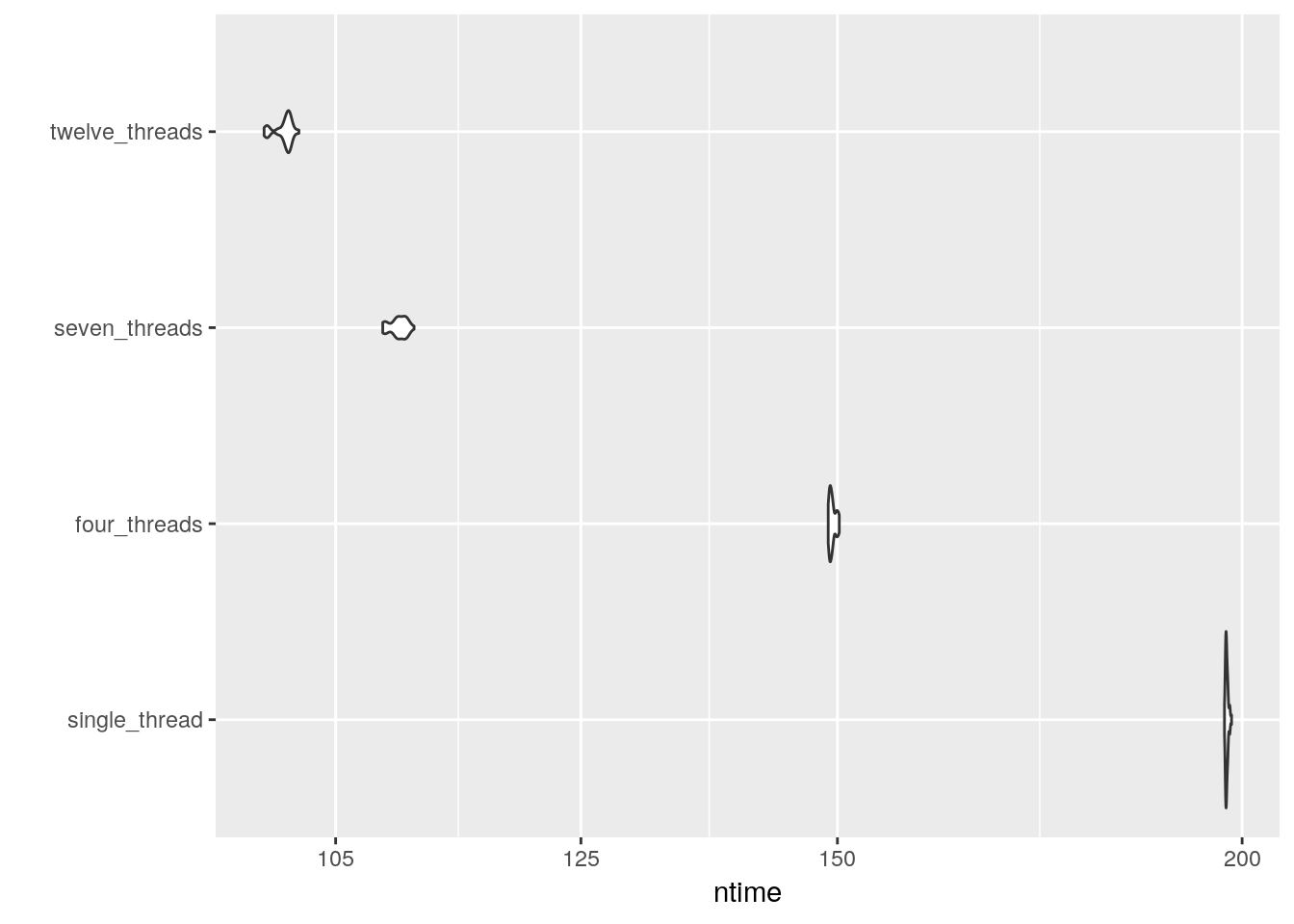
mb <- (microbenchmark(single_thread = rstan::sampling(logistic0, stan_data, chains=1, cores=1, seed=1982),
four_threads = fit_multithread(nthreads = 4),
seven_threads = fit_multithread(nthreads = 7),
twelve_threads = fit_multithread(nthreads = 12), times = 40L))autoplot(mb) + scale_y_log10(breaks=c(105, 125,150,200))